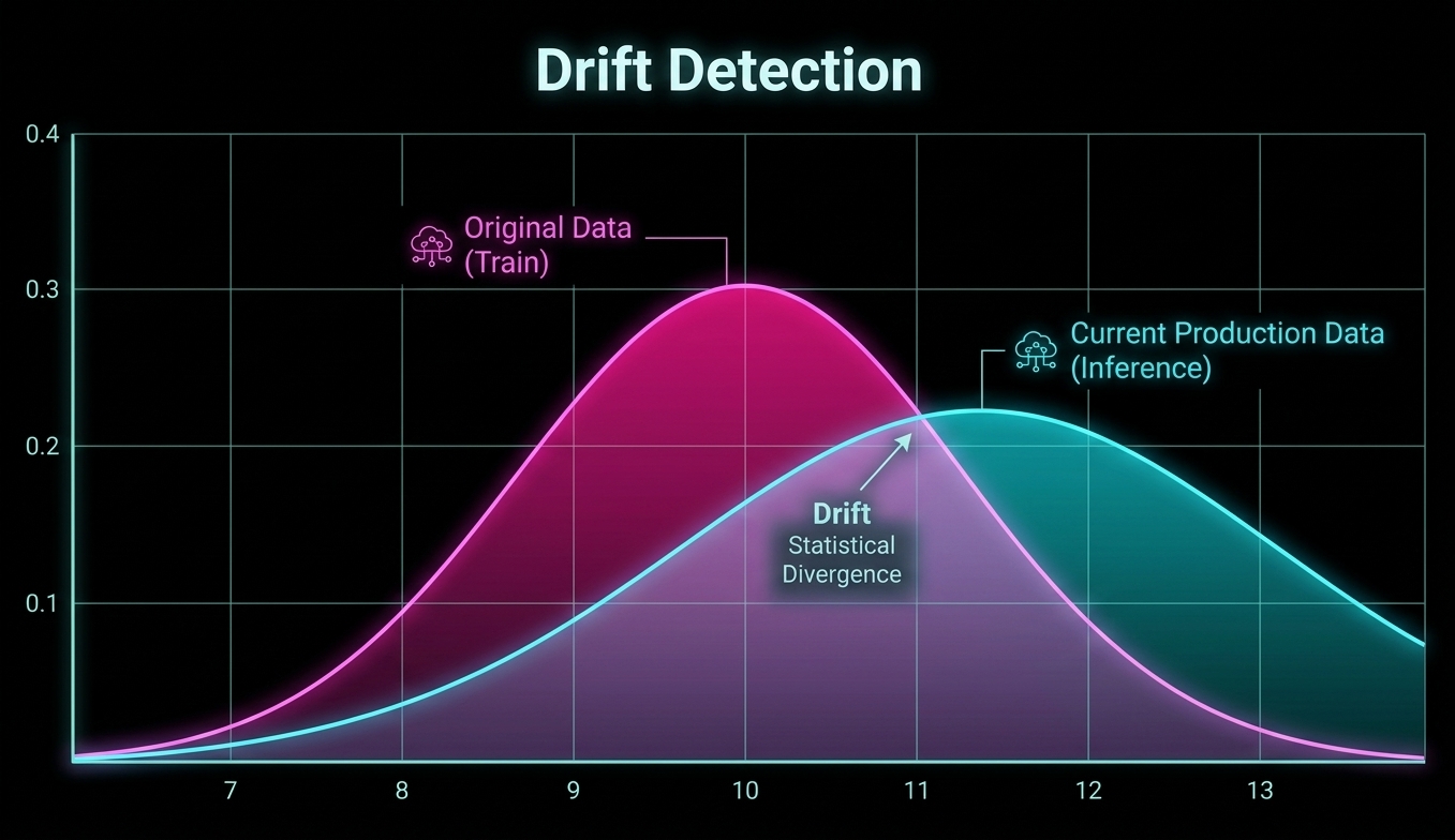
What drift actually is
Data drift is a change in the statistical properties of the input a model receives, relative to the data it was trained on. The model is unchanged. The world has moved.
It matters because models are interpolators. Within the distribution they were trained on, they perform as evaluated. Outside it, behaviour is unconstrained — and, critically, confidence does not reliably fall when it should.
Roughly 91% of ML models degrade over time, and drift is the primary mechanism.
Three types, three different responses
Conflating these leads to the wrong remediation, which is worse than none because it consumes a retraining cycle and fixes nothing.
Data drift — the input distribution changed. New product lines, new geographies, seasonal variation, new sensors, changed user behaviour. The model may still perform adequately if it generalises well; data drift is a leading indicator, not a verdict.
Concept drift — the relationship between input and correct output changed. The input distribution may be identical, but what counts as the right answer has moved. What was classified as fraud two years ago may be normal behaviour now. This is the most consequential type and the hardest to detect, because it requires ground truth.
Prediction drift — the model's output distribution changed. If a classifier historically predicted a class 12% of the time and now predicts it 31%, something has shifted even if accuracy has not visibly fallen. Requires no labels, and frequently precedes measurable accuracy loss.
The detection methods, and when each applies
Population Stability Index (PSI). Bucket the reference and production distributions, then compute the sum over bins of (actual − expected) × ln(actual / expected). Conventional interpretation: under 0.1 means no significant shift, 0.1 to 0.2 moderate, above 0.2 significant drift on that feature.
PSI's advantage is stability and interpretability — it returns the same result regardless of sample size, which makes it predictable and well suited to environments where business stakeholders act on the number. Its disadvantage is low sensitivity: it will not surface small shifts. Use it when you have a lot of data and want to react only to major changes.
Kolmogorov-Smirnov test. A non-parametric test comparing cumulative distributions for continuous features. Use the two-sample KS statistic with a p-value threshold, calibrated against expected batch size to avoid alert fatigue at scale. Highly sensitive — which becomes a liability at large sample sizes, where statistically significant differences are detected that have no practical effect.
Chi-square test. The categorical equivalent. Bucket categories, compare observed against expected counts.
Jensen-Shannon and Wasserstein distance. Smoother alternatives to KL divergence for noisy production distributions. JS is symmetric and always finite, which makes it more stable on sparse distributions than KL. KL divergence is asymmetric — the order of comparison matters, so it estimates degree of drift but drift sizes cannot be meaningfully compared against each other.
Embedding drift via cosine distance. For unstructured data — images, text, audio — feature-level statistics are not available. Compute the mean embedding for the reference and production windows, then track cosine distance between centroids with a moving-window threshold. This is the only practical approach for multimodal pipelines.
Windowed streaming detection. For continuous streams, methods like KSWIN maintain a sliding window and apply the KS test between recent and historical sub-windows, detecting change points without a fixed reference batch.
Thresholds are a starting point, not an answer
Published thresholds — PSI above 0.2, p-value below 0.05 — are conventions, not physics. Two adjustments matter in practice.
Calibrate against your own batch size. Statistical tests scale with sample size. A KS test on ten million records will flag differences with no operational meaning. Set thresholds empirically against historical batches where you know the model performed acceptably.
Confirm impact before acting. Not every drift signal requires action; confirm that distribution changes actually affect model accuracy before retraining. The strongest practice is to alert on a joint condition — input drift plus a measurable evaluation drop. Drift without evaluation impact is a false alarm and burns on-call attention.
And drift statistics are not a substitute for performance measurement. Fraud detection accuracy can fall three points in two weeks while PSI still reads as minor. The statistic is an early indicator. Performance is the verdict.
Aggregate drift hides the failure that matters
A single drift score across a dataset is nearly as misleading as a single accuracy number.
Drift is usually concentrated. One feature shifted sharply while twenty stayed stable. One category tripled in volume while the rest held. Averaged across the dataset, a serious localised shift disappears into an unremarkable number.
Two decompositions are essential: per-feature drift, so the specific input that moved is identifiable rather than inferred, and per-slice performance, so the segment where accuracy actually fell is visible. A model at 94% aggregate can be at 61% on a category representing 4% of volume — and that category is usually the rare, high-consequence one.
Without both, the alert tells you something changed but not what to do about it.
The part most tooling skips: what happens next
Detection is comparatively easy. Every monitoring product does it competently.
What follows is where the time actually goes. The conventional sequence is manual: export predictions, investigate by hand, form a hypothesis about which training data is responsible, assemble a corrective set, arrange labeling, retrain, hope. It takes weeks, produces no documentation, and is repeated from scratch on the next incident.
Retraining without diagnosis is the expensive failure mode. Retraining on more data from the same distribution that caused the failure entrenches it. And when retraining is necessary, versioning both datasets and models ensures stability and allows safe rollbacks if the new model underperforms.
A useful discipline is to build an intervention library rather than a retraining reflex — a healthy pipeline chooses among several responses based on what changed and where the risk sits.